Next: Canonical Ensemble
Up: Classical Statistical Mechanics
Previous: Classical Statistical Mechanics
This approach is suitable for obtaining the thermodynamics of a mechanically, and thermally
isolated system with fixed number of particles, volume and energy. Consider such an isolated
system, defined by -
 .
.
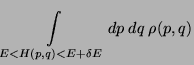
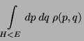
Definitions, (phase-space volume)
Therefore,
 |
(11) |
which could be written as,
if  .
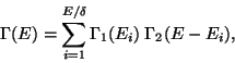
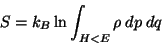
The thermodynamics, for this micro-canonical ensemble approach, is
obtained from the following equivalent definitions of the entropy,
.
The thermodynamics, for this micro-canonical ensemble approach, is
obtained from the following equivalent definitions of the entropy,
which differ only by additive constants. This recipe is meaningful only when the entropy
defined this way could be identified with the entropy defined by thermodynamics. Therefore,
we must prove that,
 is extensive, and
- is in accordance with the second law of thermodynamics.
A. - Consider an isolated system defined by ( ). Now consider two
imaginary subsystems of this system defined as,
). Now consider two
imaginary subsystems of this system defined as,
Let us assume that the interaction energy between the subsystems is very much smaller
than either  or
or  . Then,
 |
(17) |
This is true if - i) the range of inter-particle interaction is small, ii) the surface
to volume ratio for each subsystem is small. Now, the entropy for the individual
subsystems are given by,
In the composite space, spanning the entires system we must have,  and
and
 such that the phase-space is spanned by
 . Therefore, the phase-space volume of the
whole system is given by,
. Therefore, the phase-space volume of the
whole system is given by,
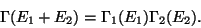 |
(20) |
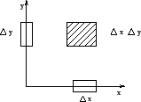
This is very much like the product space of two independent variables (for example, the
area element in the  plane, as shown in figure[2]).
Figure:
Composite Space
 |
Then, if  be the unit of energy, we have,
 |
(21) |
where the lower bound of  is zero. Therefore, the entropy of the whole system
is given by,
is zero. Therefore, the entropy of the whole system
is given by,
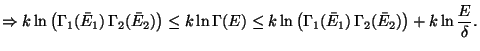
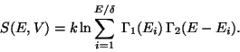 |
(22) |
Suppose,
 be the largest term in the
above series, with
be the largest term in the
above series, with
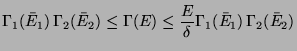
 . Then,
| |
|
 |
|
| |
|
 |
(23) |
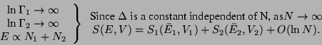
As,
 , we have,
Since,  is much slower than
  , the last term can be neglected as
 and this proves the extensive property of .
Moreover, the energies of the subsystem have definite values  and
and  such that these values maximize
 with
with  .
Therefore,
.
Therefore,
![\begin{displaymath}
\delta [\Gamma_1(\bar E_1) \Gamma_2(\bar E_2)]= 0 , \quad \mbox{with}\quad
\delta E_1 + \delta E_2 = 0.
\end{displaymath}](img76.png) |
(24) |
Therefore, it can be seen that,
![\begin{displaymath}
\delta \ln [\Gamma_1(\bar E_1) \Gamma_2(\bar E_2)]= 0,
\end{displaymath}](img77.png) |
(25) |
which implies that,
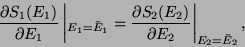 |
(26) |
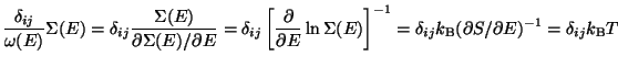
or,
 since,
 . Therefore, we conclude that
the two subsystems must have the same temperature. If this temperature scale is
now chosen to be the kelvin scale the constant is identified with the Boltzmann
constant :
. Therefore, we conclude that
the two subsystems must have the same temperature. If this temperature scale is
now chosen to be the kelvin scale the constant is identified with the Boltzmann
constant :
 . Evidently, in an isolated system,
  is the parameter
which governs the equilibrium between one part of the system with the other.
is the parameter
which governs the equilibrium between one part of the system with the other.
B. - The second law of thermodynamics states that if an isolated system
undergoes a change of thermodynamic state such that the initial and the final
states are equilibrium states, then the entropy of the final state is not smaller
than the entropy of the initial state.
Consider an isolated system defined by  . Since, the system is isolated,
and
. Since, the system is isolated,
and  are fixed. And
  can never decrease without external intervention.
Therefore, since, can only increase for an isolated system, the entropy, given
by,
can never decrease without external intervention.
Therefore, since, can only increase for an isolated system, the entropy, given
by,
 |
(27) |
also can only increase (larger volume  larger phase-space volume).
Thermodynamics using Micro-canonical Ensemble - Consider quasi-static
thermodynamics transformations where or are slowly varying. The system can
be treated using micro-canonical formulation at each instant (time-intervals small
compared to the time-scale of change) of time. The recipe is given by,
The other thermodynamic variables like temperature or pressure are obtained
the usual way, like,
 ,
,
 and so on.
The Equipartition Theorem -
Ensemble average of
 -
-
If  then
then
 .
This is the virial theorem.
.
This is the virial theorem.
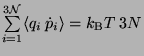
For any
 , we have,
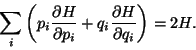 |
(31) |
Therefore, by the virial theorem, it can be seen that,
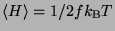 where
where
 is the number of degrees of freedom for the system. In general, if
 then
the equipartition of energy gives
then
the equipartition of energy gives
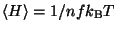 .
.
Specific Heat -
 .
Therefore, the specific heat is proportional to the number of degrees of freedom. Since,
a classical system have an infinite number of degrees of freedom, the specific heat should
go to infinity, calculated this way. The solution lies in quantum physics which tells us
that only those degrees of freedom are relevant which are excited in a particular process.
.
Therefore, the specific heat is proportional to the number of degrees of freedom. Since,
a classical system have an infinite number of degrees of freedom, the specific heat should
go to infinity, calculated this way. The solution lies in quantum physics which tells us
that only those degrees of freedom are relevant which are excited in a particular process.
Quantum Correction to  - The uncertainity principle of Quantum Mechanics tells
us that there can be no simultaneous precise measurement of a pair of canonical co-ordinate
and momenta. Hence, each
- The uncertainity principle of Quantum Mechanics tells
us that there can be no simultaneous precise measurement of a pair of canonical co-ordinate
and momenta. Hence, each  point corresponding to a particle in the phase-space is not
really a point but an area of size
point corresponding to a particle in the phase-space is not
really a point but an area of size  . Therefore, for a system of particles, the elementary
volume in the phase-space is
. Therefore, for a system of particles, the elementary
volume in the phase-space is  . Hence, the correct evaluation of
  , which is
nothing but the total number of possible micro-states accessible to the system, it should be
divided by .
, which is
nothing but the total number of possible micro-states accessible to the system, it should be
divided by .
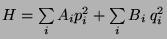
Gibbs Paradox - The Hamiltonian of a classical ideal gas of particles
is
 . Then,
where,
 . Therefore, the entropy of the ideal gas is,
 |
(33) |
This can be written as,
Consideer two ideal gases, with  and
and  particles respectivly, kept in two
separte volumes
particles respectivly, kept in two
separte volumes  and
and  at the same temperature. The change in the entropy
of the combined system after the gases are allowed to mix in a volume
at the same temperature. The change in the entropy
of the combined system after the gases are allowed to mix in a volume  is given by,
 |
(37) |
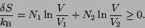
If the two gases are different this result matches with the experiment. However, if
the gases are the same there should not be any change in the entropy. The paradox was
solved by Gibbs by introducing a factor  by which should be divided in
order to produce the correct result. This comes from the fact that Quantum Mechanically
the particles are indistinguishable and therefore different microscopic configurations
are actually the same. This is known as the current Boltzmann counting.
by which should be divided in
order to produce the correct result. This comes from the fact that Quantum Mechanically
the particles are indistinguishable and therefore different microscopic configurations
are actually the same. This is known as the current Boltzmann counting.
Next: Canonical Ensemble
Up: Classical Statistical Mechanics
Previous: Classical Statistical Mechanics
Sushan Konar
2004-08-19


![$\displaystyle \frac{\delta}{\Gamma (E)} \frac{\partial }{\partial E}
\left[ \...
...eft\{ x_i ( H- E) \right\}
- \int_{H<E} dp dq \delta_{ij} (H - E) \right]$](img99.png)