Contents

• Introduction
• Preparing the data
  • Downloading the raw data
  • LTA to FITS conversion
  • FITS to MS conversion
• Data inspection
• Initial Flagging
• Flagging of non-working antennas
• Other initial flags
• Absolute flux density calibration
• Delay and bandpass calibration
• Gain calibration
• Transfer of gain calibration to the target
• Flagging on calibrated data
• Averaging data in frequency
• Imaging
• Self-calibration

Preparing the data

The GMRT data are recorded in "lta" format. To work in CASA we need to convert these into the CASA visiblity format that is called the "measurement set" (MS) format.

Downloading the raw data

From the GMRT online archive you can download data in "lta" or "FITS" format. If you downloaded the data in lta format then you will need to do the following steps to convert it to FITS format. You can download the pre-compiled binary files "listscan" and "gvfits" from the observatory.

LTA to FITS conversion

listscan fileinltaformat.lta


At the end of this a file with extension .log is created. The next step is to run gvfits on this file. gvfits fileinltaformat.log

The file TEST.FITS contains your visibilities in FITS format.

FITS to MS conversion

At this stage start CASA. A logger window will appear. The remaining analysis will be done at the CASA Ipython prompt. We use the CASA task importgmrt to convert data from FITS to MS format. In our case the FITS file is already provided so we proceed with that FITS file.

casa
importgmrt(fitsfile='uGMRT-Band4.FITS', vis='multi.ms')


The file multi.ms file contains your visibilities in MS format.

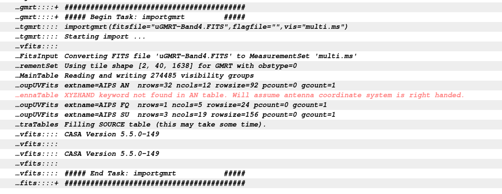
The CASA logger shows the above messages. We will ignore the warning for now.

Data inspection

The task listobs will provide a summary of the contents of your dataset in the logger window.

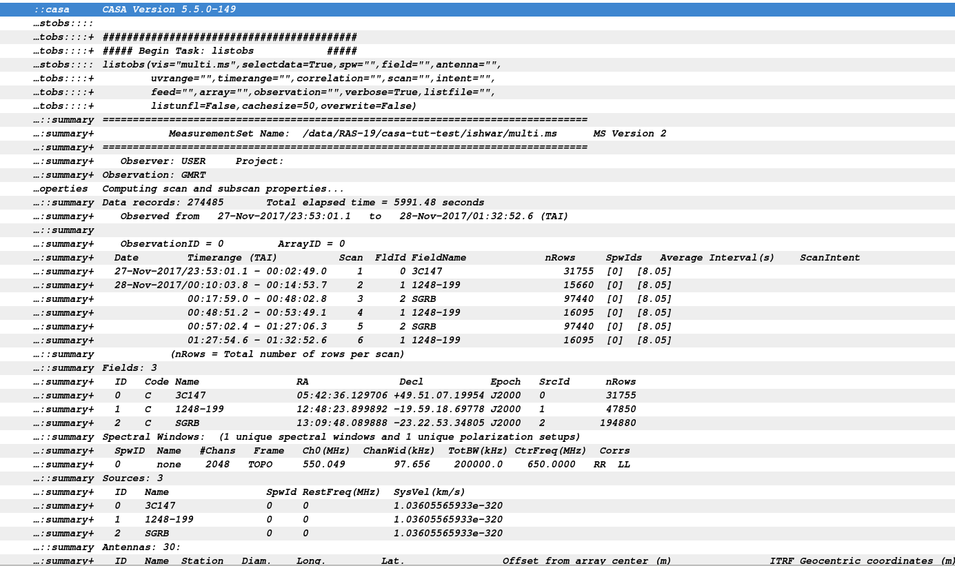
Listobs output in the CASA logger.

The task plotms can be used to plot your data. It opens a GUI in which you can choose to display portions of your data.

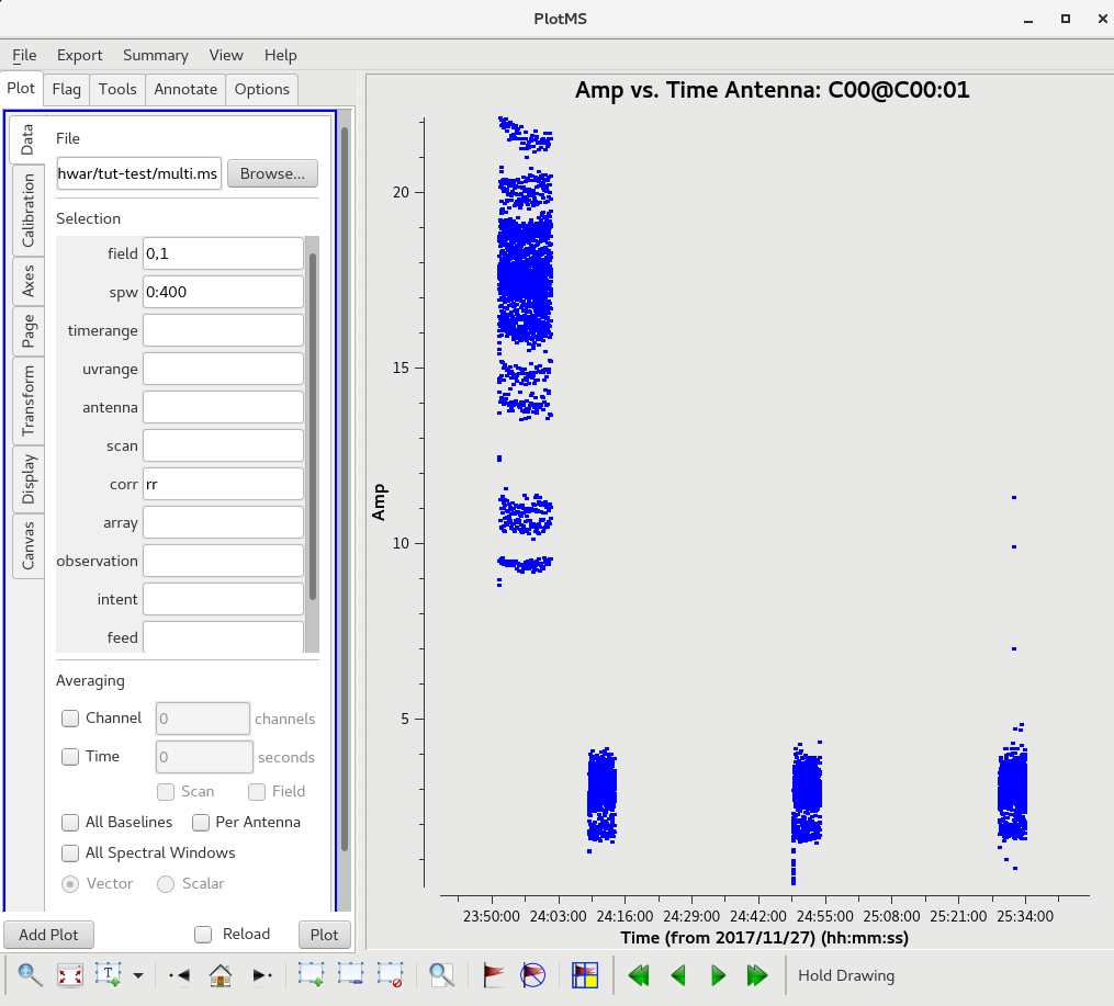
In the gui, it was chosen to plot the channel 400, 'RR' correlation for the calibrator sources (field IDs 0, 1). In the "Page" tab, iteration over "antennas" was chosen. This is how the uncalibrated amplitudes for the calibrator sources in channel 400 look for the antenna C00.

The task browsetable can be used to view your data in a tabular form.

Initial Flagging

Flagging the first spectral channel.

Flagging the first and last records of all the scans.

Using the data visualisation tasks, check if there are antennas that are not working. Non-working antennas generally show up as those having very small amplitude even on bright calibrators, show no relative change of amplitude for calibrators and target sources and the phases towards calibrator sources will be randomly distributed between -180 to 180 degreees. If such antennas are found in the data, those can be flagged using the following command.

In the test data that we are using all the antennas are working.

Automated flagging using tfcrop.

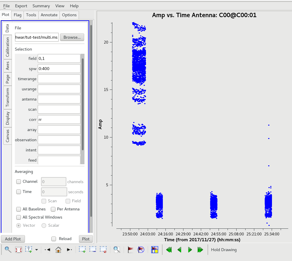
The same plot as before after the above flagging steps.

You can visualise the data (amplitude and phase) on frequency and time axes and choose to display the flagged points in a different colour. Explore the plotms GUI !

Now we extend the flags (growtime 80 means if more than 80% is flagged then fully flag, change if required)

Absolute flux density calibration

Here flux densities are set for the standard flux calibrator in the data.

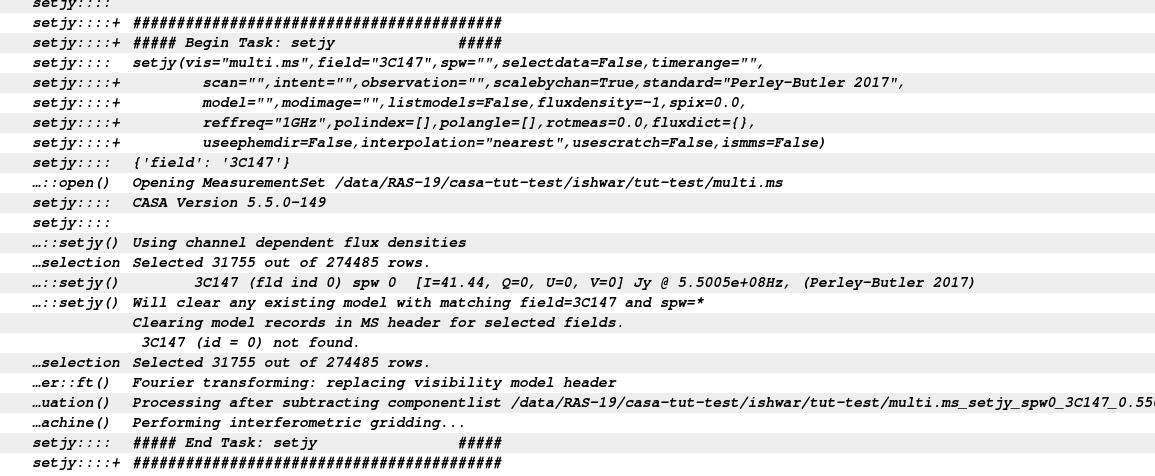
The CASA logger messages on running setjy.

If more than one flux calibrators are present, run it for each of the sources.

Delay and bandpass calibration

First we will do delay calibration. In calibration, a reference antenna is required. Here "C00" is only taken as an example. You may use any antenna that is working for the whole duration of the observation.

An initial gain calibration will be done.

Bandpass calibration using the flux calibrator.

Examine the bandpass table using plotcal.

Note the shape of the band across the frequencies. For antennas 'C00' and 'E04' note that the feeds at the GMRT were not upgraded to the new wideband feeds at the time of the observations and therefore have a narrower range of channels with high gains. We will flag the channels with low gains for these antennas.

default(flagdata)
flagdata(vis='multi.ms', mode='manual', field ='', spw='0:0~170,0:990~2047', antenna='C00', timerange='', correlation='') default(flagdata)
flagdata(vis='multi.ms', mode='manual', field ='', spw='0:0~170,0:990~2047', antenna='E04', timerange='', correlation='')

Gain calibration

An final gain calibration will be done.

Transfer of gain calibration to the target

First apply calibration to the amplitude and phase calibrators.

Calibrate the target.

In this step the "corrected" data column is created in the MS file.

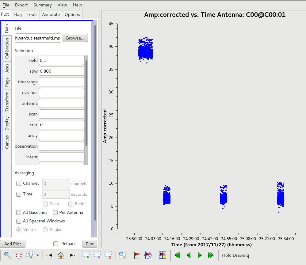
The calibrated Amp Vs Time for the calibrators.

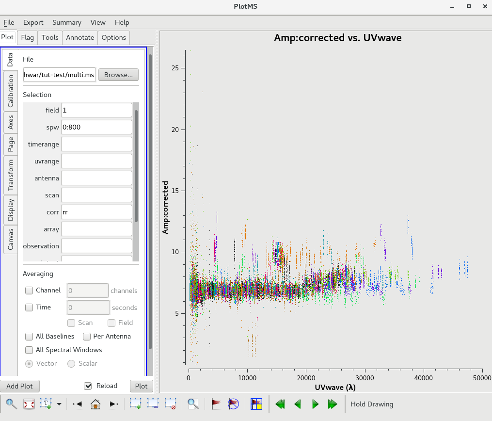
The calibrated Amp Vs UVWAVE for the calibrator 1248-199.

Use plotms to locate which antennas and baselines have the outlier data. Use the task flagdata to flag that data. Here examples of additional flagging are shown.

Flagging of antenna S04.

default(flagdata)
flagdata(vis='multi.ms', mode='manual', field='', spw='0', antenna='S04', correlation='', action='apply', savepars=True, cmdreason='badant')

Flagging of the baseline C04-E03.

default(flagdata)
flagdata(vis='multi.ms', mode='manual', field='', spw='0', antenna='C04&E03', correlation='', action='apply', savepars=True, cmdreason='badbl')

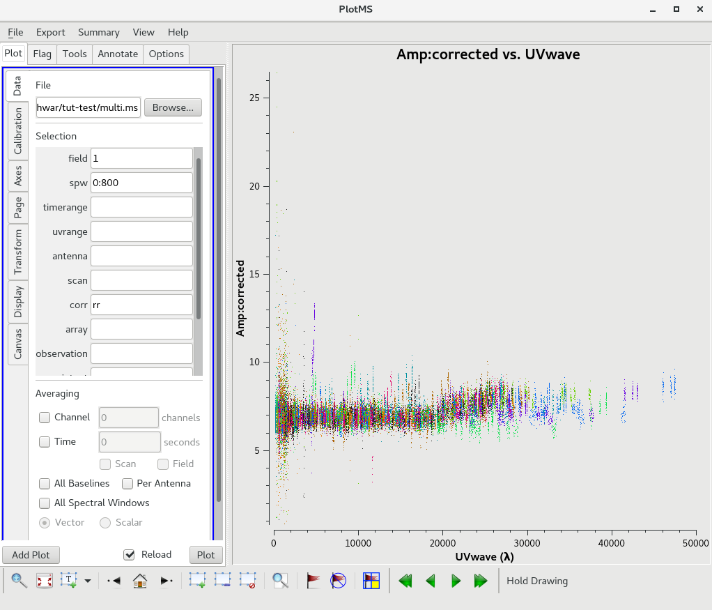
The calibrated Amp Vs UVWAVE for the calibrator 1248-199 after additional flagging.

We will split the calibrated target source data to a new file and do the subsequent analysis on that file.

Flagging on calibrated data

In this section flagging is done on calibrated target source data.

The calibrated target data before (left) and after (right) flagging.

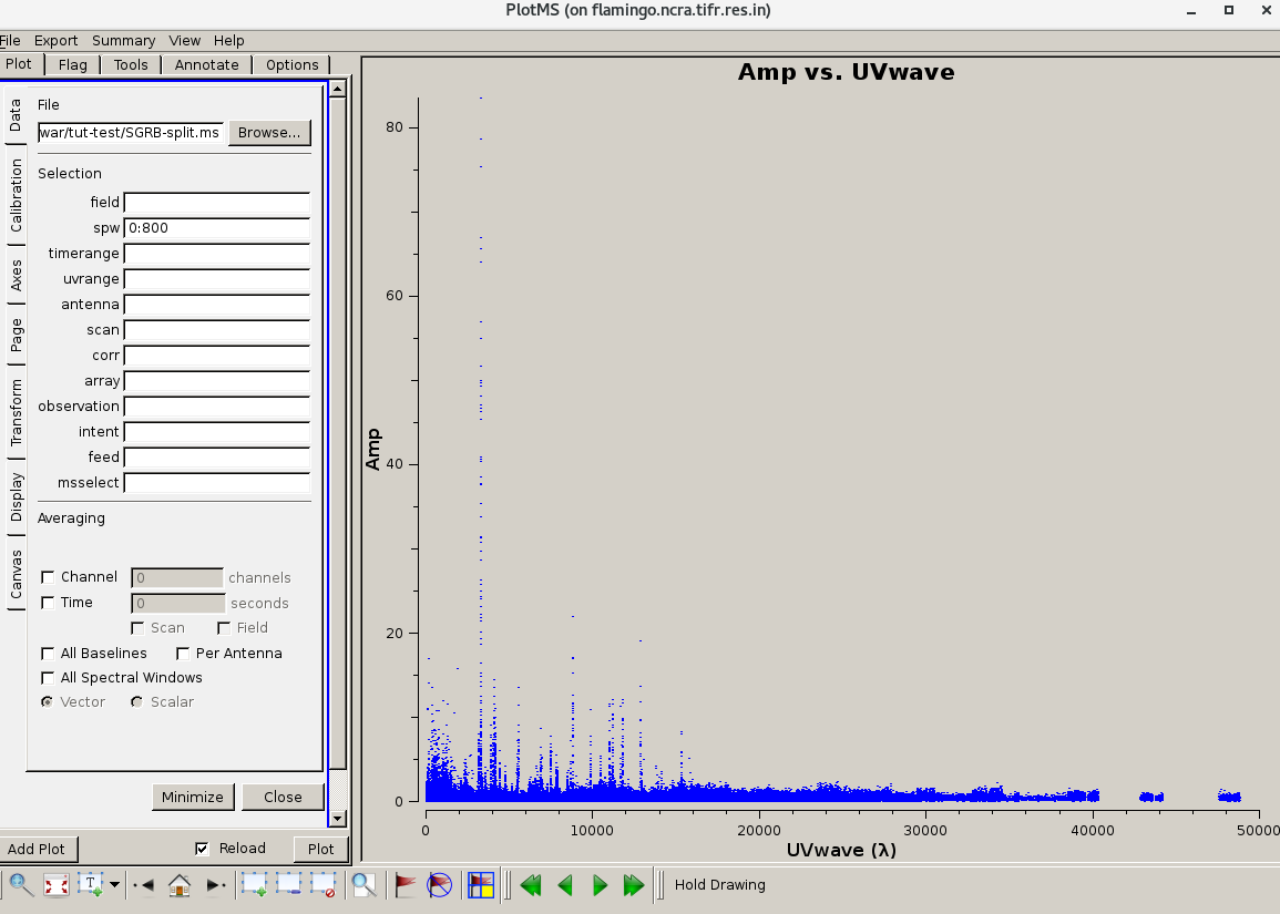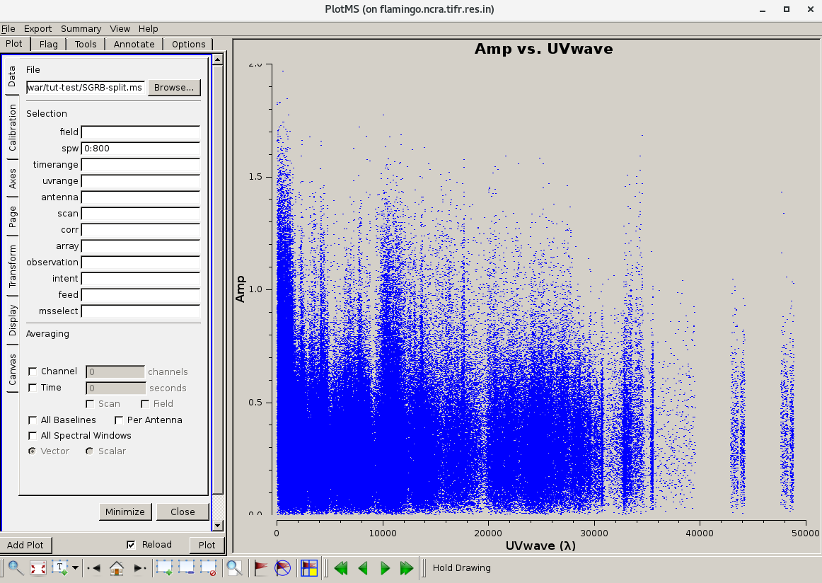Now extend the flags (80% or more means full flag, change if required)

default(flagdata)
flagdata('SGRB-split.ms',mode="extend",field='',datacolumn="data",clipzeros=True,spw = '', ntime="scan", extendflags=False, extendpols=False,growtime=80.0, growfreq=80.0,growaround=False, flagneartime=False, flagnearfreq=False, action="apply", flagbackup=True,overwrite=True, writeflags=True)

Averaging in frequency

The data are averaged in frequency to reduce the volume of the data. However the averaging is done only such that one is not affected by "bandwidth smearing". For Band 4 it is recommended to average up to 10 channels (when BW is 200 MHz over 2048 channels). However in order to keep the computation time reasonable, for this tutorial we will average 20 channels.

Some more flagging may be done on the data at this stage. Depending on your science goal you should use a flagging strategy. Here only an example is given.

default(flagdata)
flagdata(vis='SGRB-avg-split.ms',mode="tfcrop", datacolumn="data", field='', antenna='',spw = '', ntime="300s", timecutoff=5.0, freqcutoff=5.0, timefit="poly",freqfit="line",flagdimension="freqtime", extendflags=False, timedevscale=5.0,freqdevscale=5.0, extendpols=False,growaround=False, action="apply", flagbackup=True,overwrite=True, writeflags=True) default(flagdata)
flagdata(vis='SGRB-avg-split.ms',mode="rflag",datacolumn="data",field='', timecutoff=5.0, antenna='',spw = '', ntime="300s", freqcutoff=5.0,timefit="poly",freqfit="poly",flagdimension="freqtime", extendflags=False, timedevscale=5.0,freqdevscale=5.0,spectralmax=500.0,extendpols=False, growaround=False, flagneartime=False,flagnearfreq=False,action="apply",flagbackup=True,overwrite=True, writeflags=True)
default(flagdata)
flagdata('SGRB-avg-split.ms',mode="extend",field='',datacolumn="data",clipzeros=True,spw = '', ntime="300s", extendflags=False, extendpols=False,growtime=80.0, growfreq=80.0,growaround=False, flagneartime=False, flagnearfreq=False, action="apply", flagbackup=True,overwrite=True, writeflags=True)

Imaging

We will use the task tclean for imaging. To save on computation, in this example we have set wprojplanes=128. In general to account for the w-term more accurately set wprojplanes= -1 so that it will be calculated internally in CASA. In this example we have used "interactive = False" in tclean. You may choose to do an "interactive = True", put the boxes on the sources you want to deconvolve manually to learn the process.

You can view the image using the "viewer". You can also view the rest of the images created by tclean - the .psf, .mask, .model.

The first image - the entire image is shown. Due to the effect of the primary beam you can see that there are many sources at the centre.

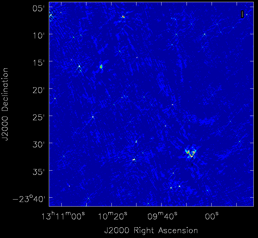
A zoom-in on the central region of the first image.

Self-calibration

This is an iterative process. The model from the first tclean is used to calibrate the data and the corrected data are then imaged to make a better model and the process is repeated. The order of the tasks is tclean, gaincal, applycal, tclean. A reasonable choice is to do 5 phase only and two amplitude and phase self-calibrations. We start from a longer "solint" (solution interval), for e. g. "8min" and gradually lower it to "1min" during the phase only iterations. For "a&p" self-calibration, again choose a longer solint such as "2min". We keep solnorm=False in phase only iterations and solnorm=True in "a&p" self-calibration. As the iterations advance, the model sky is expected to get better so in the task tclean, lower the threshold and increase niter.

Using the task "plotcal" you can examine the gain table. In successive iterations of self-calibration, you should find that the phases are more and more tightly scattered around zero. If this trend is not there, you can suspect that the self-calibration is not going well - check the previous tclean runs to see if the total cleaned flux was increasing.

We will split the corrected data to a new file and use it for imaging. This is just for better book-keeping.

In the next iteration we will use a larger niter and lower the threshold. In the tclean messages do check the total cleaned flux and the number of iteration needed to reach that.

default(tclean)
tclean(vis='vis-selfcal-p1.ms', imagename='SGRB-img-1', selectdata= True, field='0', spw='0', imsize=9000, cell='1.0arcsec', robust=0, weighting='briggs', specmode='mfs', nterms=2, niter=3000, usemask='auto-multithresh',minbeamfrac=0.1, smallscalebias=0.6, threshold='0.5mJy', pblimit=-1, deconvolver='mtmfs', gridder='wproject', wprojplanes=128, wbawp=False, restoration = True, savemodel='modelcolumn', cyclefactor = 0.5, parallel=False, interactive=False)

Repeat until you stop seeing improvement in the image sensitivity.

After you get your final image you need to do a primary beam correction. The task "widebandpbcor" in CASA does not have the information of the GMRT primary beam shape. A new task has been written for that. You can refer to uGMRT primary beam to get that task and follow the instructions with it to do a primary beam correction for your data.